Geometry Layers
Introduction
This chapter brings you the specification of geometric layers that you can add to
the chart. In Stagraph 1.1 you can use 41 geometric layers. The following text
describes how you can add them to data visualization, what aestetic properties
you can define and how to setup positional and other specific properties.
Each geometry layer forms a relatively simple object with several adjustable
properties (arguments). Combining these geometric layers, you can create very
impressive data visualization relative quickly and easily.
In addition to geometric layers, program allows you add also statistical layers
(more in chapter Statistical Layers). If you want to add a new layer into plot,
display the ribbon toolbar tab, named Layers.
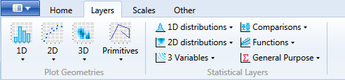
Under the four buttons in the Plot Geometries group are logically divided geometry
layers with which you can work. The second option how to add objects into your chart
is by choose from contextual menu in the Plot panel.
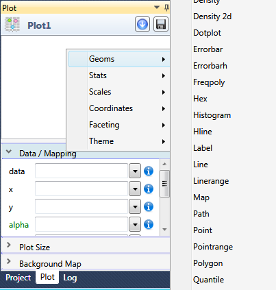
All items in contextual menu are displayed (oppsed to the ribbon toolbar) in alphabetical
order. It is up to you which method you preffer (context menu or ribbon toolbar). I prefer
the context menu (besause of speed).
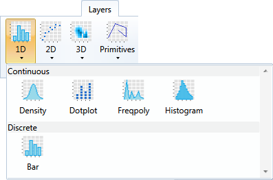
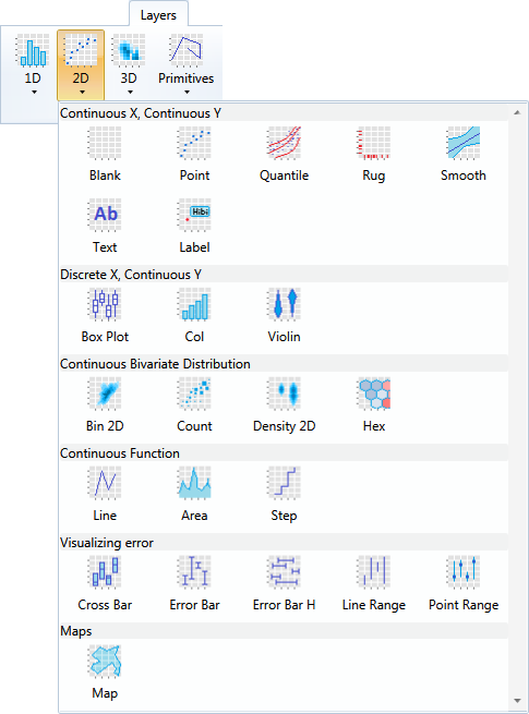
As has been said, geometries are in the ribbon toolbar divided into four logical groups.
The first gourp are geometries under the 1D button. These objects required for basic
rendering only one position aesthetic (x). From this menu you can add geometries for
density plot, dotplot, frequency plot, histogram and barplot.
The second group (under the 2D button) forms geometries that are based on two position
aesthetics (x and y). These are in menu divided by the character of its position scales
(dicrete or continuous). After click, selected geometry is added into plot that is
currently displayed in the Plot panel. Using these geometries it is possible to create
scatter plot, you can add labels, quantile regression lines, boxplots, violins, bars,
lines, areas, error bars or map layers.
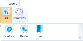
The third group (3D) consists of three geometries that must be defined by three aesthetics
(x, y, z or by x, y and color). With these geometries you
can create contour plot, raster plot or tile plot.
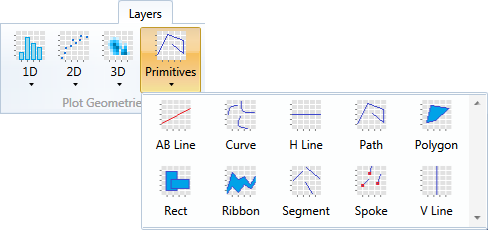
The last group of geometries is hidden under the Primitives button. Here are simple (help)
geometries with which you can enrich your data visualization, such as AB lines, curves,
horizontal and vertical lines, polygon, path, line segment or ribbon geometry.
Geometries that you put into the visualization are shown in the top part of the Plot panel.
If you select one of these geometries by mouse, its properties will be displayed at the
bottom panel part.
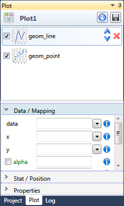
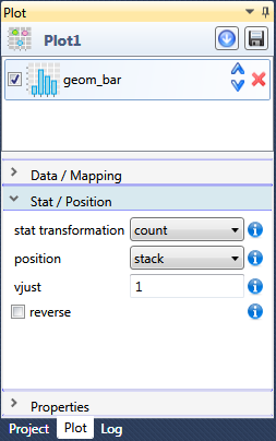
The properties of geometry objects are divided into three sections. In the first section
(Data / Mapping) you can define dataset that will be used for geometry and individual
customizable aesthetics. In the second section (Stat / Position) you can setup a statistical
transformation of dataset and edit position properties. Finally, in the last section
(Properties) are listed other settings for geometry display modification.
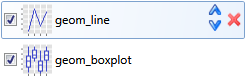
If you add several geometries into plot, they are drawn in the order as they were inserted.
If you want to change their rendering order, you can do it using buttons that appears when
you select some geometry. It is also possible to remove geometry using the Remove button.
If you want to deactivate object in plot (without removing), use the check-box before the
object icon.
The program (in version 2.0) includes more than 80 types of geometries that you can use for your data visualizations.
Geometry aesthetics
If you select in the Plot panel one of inserted geometry layer, in the
bottom panel part will show its properties that you can setup. In the
first section, named Data / Mapping, you can choose a dataset that will
be used and then you can define several aesthetic properties.
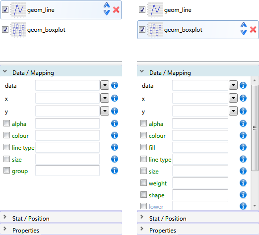
List of available aesthetic properties is slightly different for
each geometry layer. More complex geometry contains more aesthetic
properties. Individual aesthetic properties have identical options
across geometries and its description is content of separate chapter,
where you can find all the necessary information for their full
utilization. Examples of their setup can be found also in chapters
describing individual geometries.
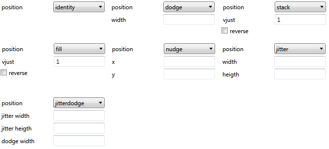
Position Property
In the second section (Stat / Position) is a property position that is
described in this chapter. Position property can be used to fine tune
positioning of objects to achieve effects like dodging, jittering or stacking.
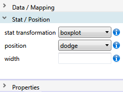
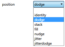
Overall, you can define in Stagraph seven types of position options.
Each geometry layer has defined some position by default. For example,
geom_point have set this property to identity, which means that all points
are displayed at exactly defined position. In contrast, geom_bar has
defaultly set position to stack and bars are stacked each other.
If you change this property using the Position combo-box, help settings
displays for selected option. Only the identity position does not have
any additional properties.
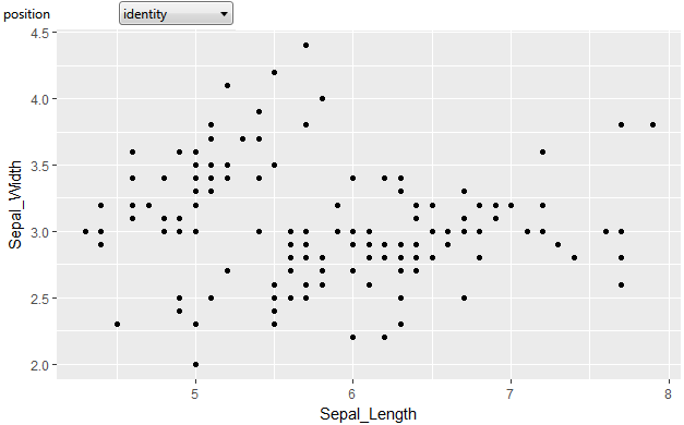
As first, the identity position will be described. This position is the
default for multiple geometries, such as geom_point or geom_line. The
values are rendered as defined by positional aesthetic properties (x, y).
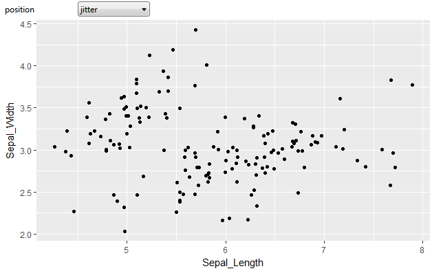
The second type of position is jitter. As an example, we can use the
previous chart, where the position property is set to identity and
more points are not visible because they overlap. If we change the
position to jitter, geometric objects are a little bit moved (randomly),
so they do not overlap. For this position option you can set two properties
(width, height) that defines maximum shift in the range from 0 to 1. A
value of 1 means the jitter values will occupy 100% of the implied bins.
If you enter 0, the geometry will not move in a given direction. An
example is shown in the following figure.
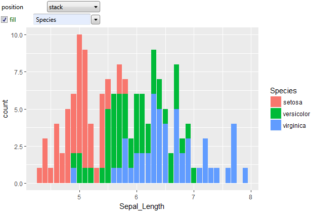
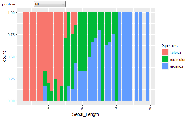
Another two position properties stack and fill overlaps objects on top
of aech another. The fill type of positioning stacks bars standardizes
each stack to have constant height. Example of these setting is displayed
in following two figures. In addition, if you use these options, you can
setup two properties – vjust and reverse.
The vjust property is useful if you use geoms that are used for position
(geom_point or geom_line) and not dimension (geom_bar, geom_area). You can
set this property as numerical value from 0 to 1. If you set this value
to 0, objects will be aligned with the bottom. At value 0.5 will be aligned
with middle and at 1 (default setting) for the top.
Complete documentation for each type of position you can see if you display
integrated R Console and write the command that begins with question mark,
followed with “position_” and ends with the name of the position option.
For example:
?position_stack
Another type of position that you can select is dodge. This position
preservers the vertical position of gemometry objects while adjusting
the horizontal position. In this way you can see next to each other
several geometries that would be otherwise overlapped (e.g. boxplots).
This position is often used when the X-axis shows categorical values.
An example of such position setting is shown in the following figure.
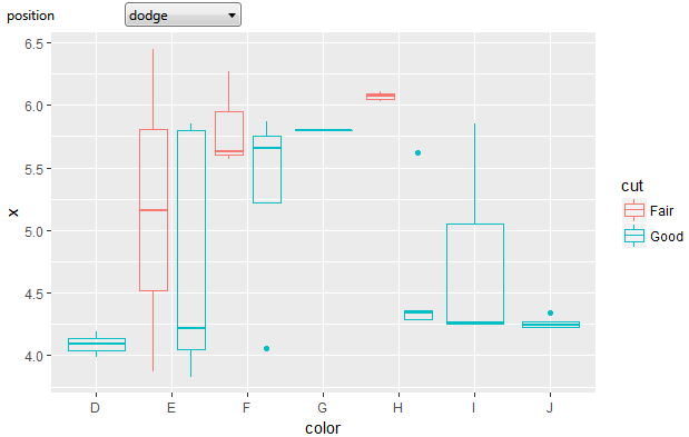
For each category on the X-axis are shown two boxplots that are based
on the color aesthetic property, mapped to dataset variable cut. For
this position, you can define help property width as numerical value
in the range from 0 to 1. This parameter defines the width of area in
which will be your geometries dodged. At 1, geometries occupy the entire
width of available area. If you set 0.5, geometries consume only half width
and will be visually separated (for each X category).
Next position option – jitterdodge combines jitter and dodge position into
one. Imagine the viewing points on the categorical X axis, where points are
dividided according to another categorical variable (e.g. color aesthetic).
If you want to divide them in the space (dodge), while ensuring that they do
not overlap (jitter), you will use exactly this position type. An example is
given in the following figure.
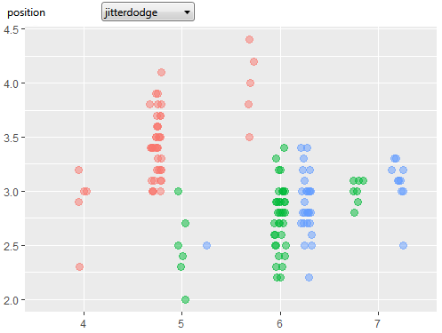
For this position option, you can adjust three help properties. Properties
jitter width and jitter height serves for definition of jitter degree in x
and y direction. The range for these values is defined as in the case of
jitter position. For the dodge amount in the x direction (default 0.75)
we use dodge width property. This position option is frequently used for
display of boxplots (posision_dodge) with all measurements in the form of
points (position_jitterdodge).
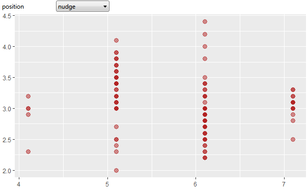
Finally, the last type of position stayed – nudge. This type is used
if you want to use geom_text or geom_label along with geom_point geometry.
Frequently we need to move little our text labels for resolve the geometries
overlap. In this case, we can choose the nudge position and using the help
properties x and y we can set exact shift of selected geometry layer in one
or both directions. The following figure shows an example of this position
option. On the X-axis, we used integer variable with point geometry. These
points we shift slightly to the right from their real integer position.
The best way how to understand these position options (with all help
properties) is to use them at work. I recommend using several geometries,
such as geom_point, geom_bar, geom_text or geom_boxplot and testing their
functionality on real examples. Remember that every geometry layer has
defaultly set one of these position options.
In the following section, we will introduce statistical transformations of
data before the final visualization.
Statistical Transformation
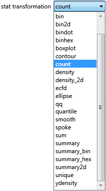
Another very important property for data visualization is selected
statistical transformation. This property is located in the Plot
Panel, section Stat / Position. Basically this property determines
transformation of input data into the form needed for proper visualization.
Every geometry layer has predefined some statistical transformation. The
default setting for several geometries is identity. If your geometry has
choosen this option, data are used and displayed without any statical
preprocessing as they are stored in the dataset. An example would be geom_point.
In this case, in the final data visualization are used as position aesthetics
variables from the dataset.
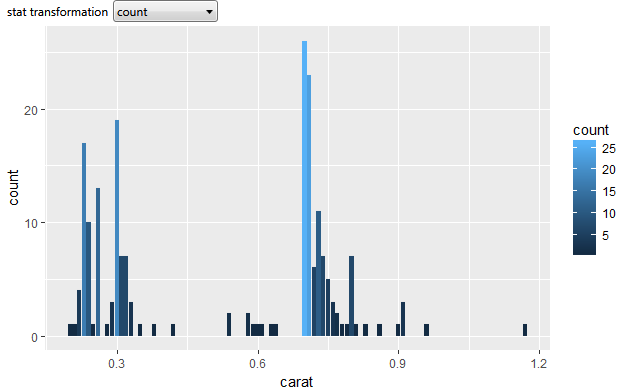
Other geometries have predefined different statistical transformations.
For example, geom_bar has the count option choosed. This means that your
data will be displayed as count (Y axis) of unique (or binned) X values.
Overall, the program offers 32 statistical transformations.
Very important functionality of the program is that you can change the
predefined statistical transformation. In this way, you can use any
geometry and combine them into your desired shape or you can create
entirely new (atypical) data visualization. If the statistical transformation
is set (other than identity), new varaibles are created, based on used
aesthetical properties.
For example, if the statistical transformation is set to count, the program
calculates a new variable named count, which will include a number of values
for each unique X variable. These automatically generated variables are named
computed values and you can work with them – you can map them to aesthetic
properties. More about their practival use is in chapter Aesthetic Properties –
Intro.
The following three pictures show the geom_bar geometry with different
statistical transformation settings. By default, geom_bar has set the
statistical transformation to count. In this case, program transforms
used data into two varaibles – unique x values (or bins) and number of
its occurrence in dataset.
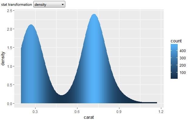
If you change statistical transformation to density, program calculates
for defined positional aesthetic the kernel density estimate.
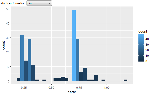
If you set the statistical transformation to the bin, program calculates
number of observations in each bin and displays its coutns as bars. An
example is shown in the following figure. This statistical transformation
is useful if you have on the X-axis continual data. For disrete data is
more appropriate the count transformation.
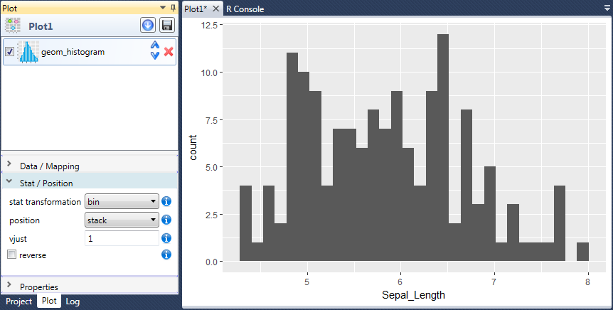
In the second example we will shiw how you can use one statistical
transformation in different geometry layers. As an example can be
used geom_histogram. This geometry is basically geom_bar layer with
bin as the default stastitical transformation. This transformation
split continual X scale into several segments and in these segments
counts all observations – classical histogram. An example is displayed
in the following figure.
What if you want to see calculated results using different geometries?
An example is shown in the following figure. In this case, histogram
values are displayed using three geometries – geom_line, geom_step and
geom_point. The only thing you must to do is to map in each geometry
layer the x position aesthetic to Sepal_Length variable and set the
statistical transformation to bin. Subsequently program calculates base
values for histogram and display them parallelly using multiple geometries.
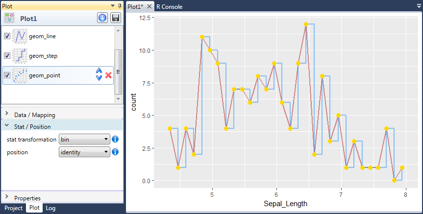
In this way, you can combine together statistical transformations and
geometries. The result can be very unusual and impressive visualizations
of your data. In the following text are briefly introduced all statistical
transformations that can be used in relation to geometries.
Other Properties
The first and second sections of layer properites (in Plot panel) are for
dataset selection, easthetics properties mapping, statistical transformation
choosing and to adjust the positioning properties. The last section (named
Properties) includes two types of settings. The last three items are the
same for all geometries. All other properties included in this section are
specific to the selected geometry. For example, geom_point does not include
any other specific settings and therefore in the Properties section are only
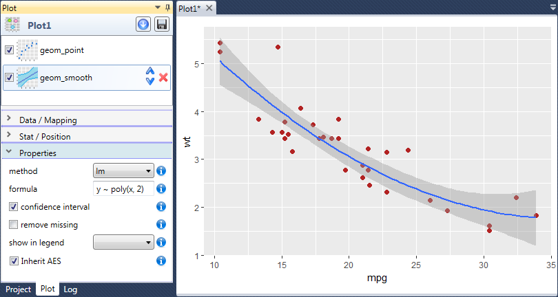
three basic items. Conversely, geom_smooth contains in this section three
other properties that are specific only for this geometry.
The first property that occurs in all geometries is a check-box named
remove missing. If this check-box is set to FALSE, missing values are
removed with a warning (in the Log panel). If TRUE, missing values are
silently removed.
The second property show in legend defines whether the given layer will be
included in legend. For example, in the previous figure the fill color scale
is not displayed in legend, because we set the property to FALSE.
Finaly the check-box Inherit AES remains. If FALSE, overrides the default
aesthetics, rather than combining with them. This is most useful for helper
functions that define both data and aesthetics and shouldn’t inherit behaviour
from the default plot specification, e.g. borders.
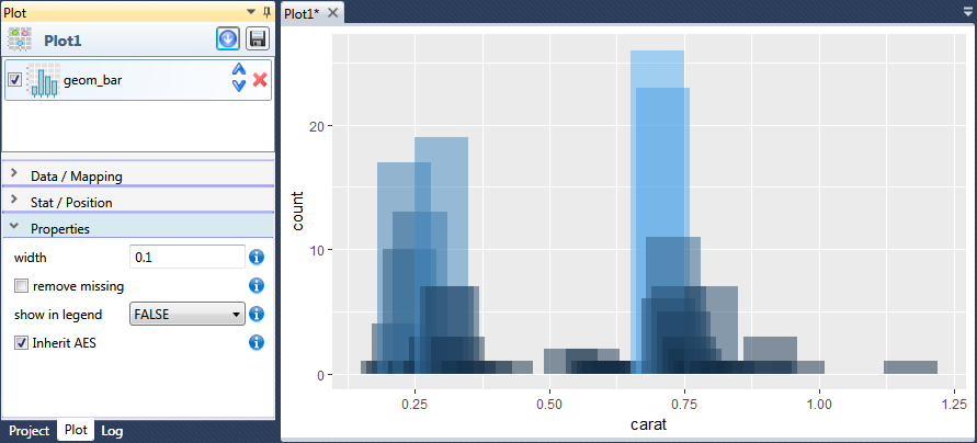
Other properties that are shown in this section allow you to set specific
properties of selected geometry layer. For example, in the previous figure
we set the width property to used-defined value. Several specific properties
has, for example, geom_smooth layer, which is displayed in the following
figure. geom_smooth includes adjustable properties method, fomula and
confidence interval. More about these specific properties will be in the
following chapters, along with real examples of use.