geom_density
Computes and draws kernel density estimate, which is a smoothed
version of the histogram. This is a useful alternative to the
histogram if for continuous data that comes from an underlying
smooth distribution.
Aesthetics
Other Properties
| bw |
the smoothing bandwidth to be used. If numeric, the standard deviation of the smoothing kernel. If character, a rule to choose the bandwidth, as listed in bw.nrd |
| adjust |
a multiplicative bandwidth adjustment. This makes it possible to adjust the bandwidth while still using the a bandwidth estimator. For example, adjust = 1/2 means use half of the default bandwidth |
| kernel |
kernel. See list of available kernels in density |
| trim |
this parameter only matters if you are displaying multiple densities in one plot. If FALSE, the default, each density is computed on the full range of the data. If TRUE, each density is computed over the range of that group: this typically means the estimated x values will not line-up, and hence you won't be able to stack density values |
Computed Variables
| density |
density estimate |
| scaled |
density estimate (scaled to maximum of 1) |
| count |
density * number of points (probably useless for violin plots) |
Similar Geometries
geom_histogram,
geom_freqpoly,
geom_violin
Description and Details
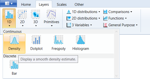
Using the described geometry, you can create density plot that is
defined by one positional aesthetic property (x). You can find
this geometry in the ribbon toolbar tab Layers, under the 1D button.
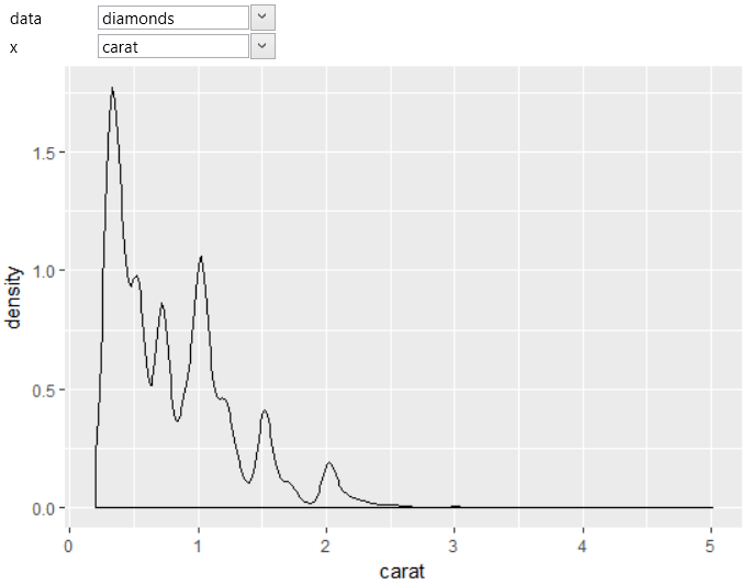
If you want to create a density plot, you use the geom_density
geometry layer. For the following examples, we will use the
built-in diamonds dataset. For density plot, you must define
the variable that will be used for the x positional aesthetic
property. In our case, we used for this purpose a continuous
variable carat. The resulting density plot is shown in the
following figure.
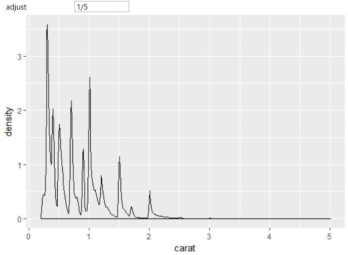
You can set multiple properties within the geom_density layer.
One of them is the adjust property – multiplicative bandwidth
adjustment. Default value is set to 1. The following figure
shows how the density plot changes when the adjust property
is reduced.
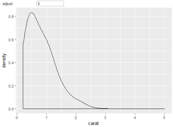
Conversely, the next plot shows how the density plot changes
if we increase the adjust value from default 1 to 5.
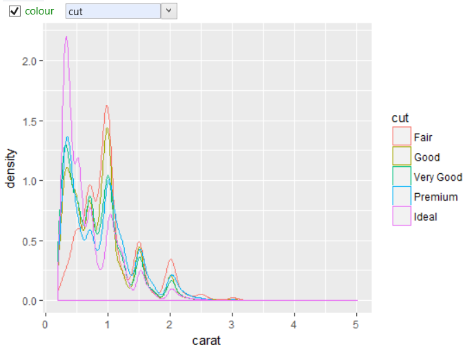
As with other geometries, you can work with multiple aesthetic
properties. In the following example, the color aes was mapped
to a categorical variable cut that identify the quality of
diamonds. The dataset is divided into individual groups according
to the selected variable and the density plot is processed for
each group individually. As a result, these lines are color-coded
using the selected variable (cut).
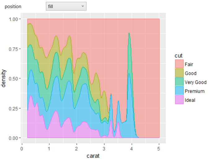
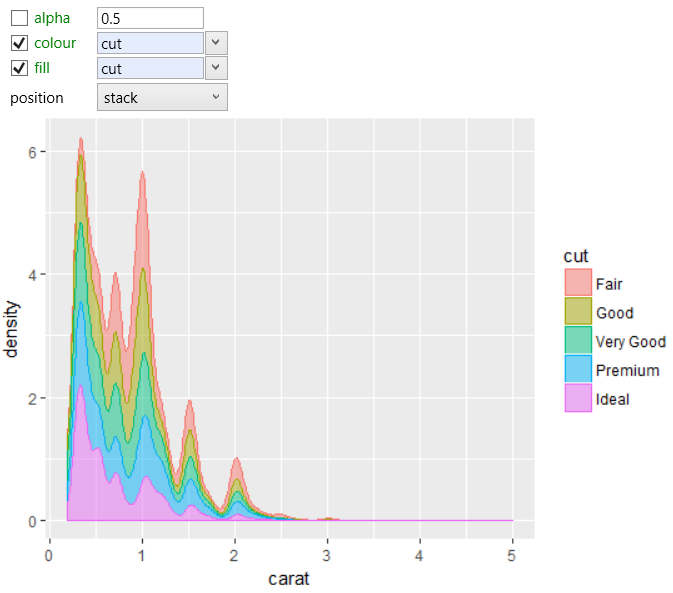
The following graph shows the same density plot, where the
fill property was mapped also to the same variable (cut)
and the alpha parameter was set to 0.5. In addition, for
better readability, we changed the position property to
stack so the individual lines are stacked on each other.
For the last example, we used the same settings and only
changed property was position. Here we choose the fill
option and the result is shown in the following chart.