 geom_smooth
geom_smooth displays patterns in the presence of overplotting.
Aesthetics
Other Properties
| bins |
numeric vector giving number of bins in both vertical and horizontal directions. Set to 30 by default |
| method |
smoothing method – function to use, e.g.
"lm",
"glm",
"gam",
"loess",
"rlm".
For method = "auto" the smoothing method is chosen based on the size of the largest group (across all panels). loess is used for less than 1,000 observations; otherwise gam is used with formula = y ~ s(x, bs = "cs"). Somewhat anecdotally, loess gives a better appearance, but is O(n^2) in memory, so does not work for larger datasets |
| formula |
formula to use in smoothing function, eg. y ~ x, y ~ poly(x, 2), y ~ log(x) |
| se |
display confidence interval around smooth? TRUE by default, see level to control |
Computed Variables
| y |
predicted value |
| ymin |
lower pointwise confidence interval around the mean |
| ymax |
upper pointwise confidence interval around the mean |
| se |
standard error |
Similar Geometries
geom_quantile
Description and Details
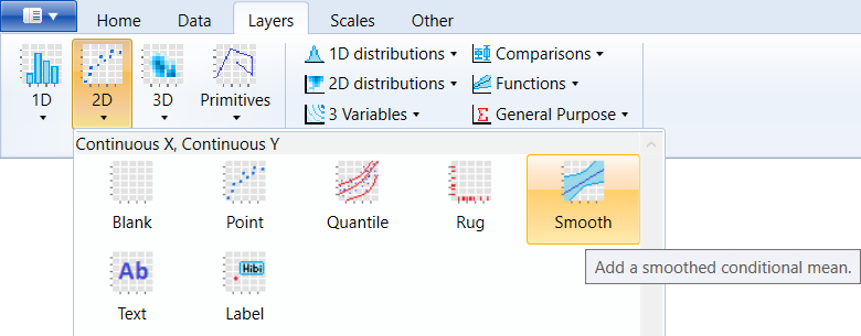
Using the described geometry, you can insert a geometric
object into your data visualization – smoothing line that
is defined by two positional aesthetic properties. You
can find this geometry in the ribbon toolbar tab Layers,
under the 2D button.
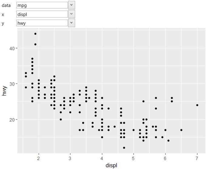
You can use the geom_smooth layer to look for patterns in
your data. We use this layer to Plot two continuous
position variables in the graph. The basic setting for
described geometry is shown in the following plot. We will
show an example on the built-in mpg dataset, from which we
will display the relationship between the displ and hwy
variables. At the beginning, we use the visualization with
the point geometry.
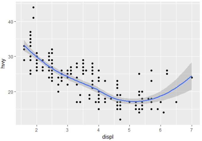
In the same way (using two positional aesthetics), we define
geom_smooth geometry. The result of this setting is shown
in the following figure. The regression line is rendered
by default in blue and confidence intervals are denoted
by gray.
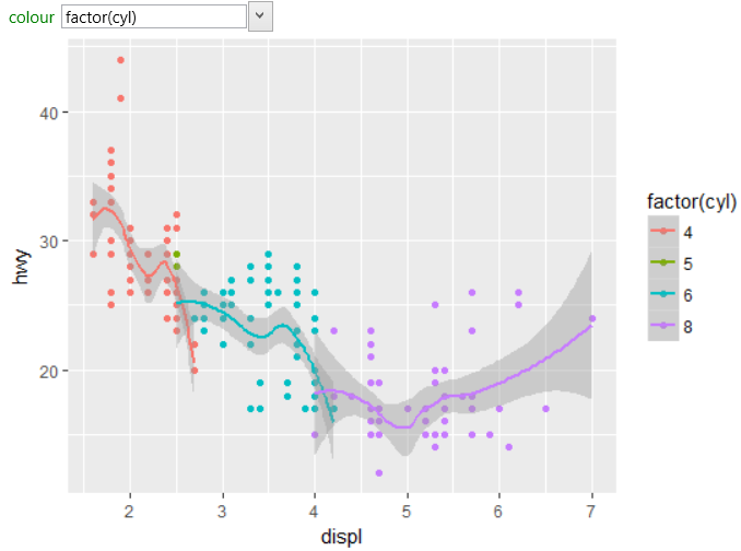
As with other geometries, you can work with several
aesthetic parameters. The following graph shows an
example of using the color property that we mapped
to categorical variable factor(cyl). As a result of
this setting, the dataset was divided by this variable
to four groups and individual smooth lines were created
for these sub-datasets.
By default, the
loess or
gam
function is used for
smoothing (in relation to the size of dataset).
Using the method combo-box, you can change this
function to
lm,
glm,
gam,
loess,
rlm.
By the
formula property you can set the formula that will
be used in the smoothing function. The most common
formulas you can find in the property context menu:
y ~ x and y ~ poly(x, 2) or y ~ log(x). According
to these two settings, it is possible to redefine
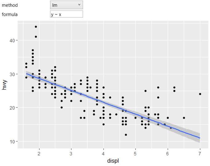
the smoothing function. In the following example,
we changed the method to lm (linear model) and left
the formula in the base shape (y ~ x). The result
represents the basic linear smoothing of the relationship
between the displ and hwy variables.
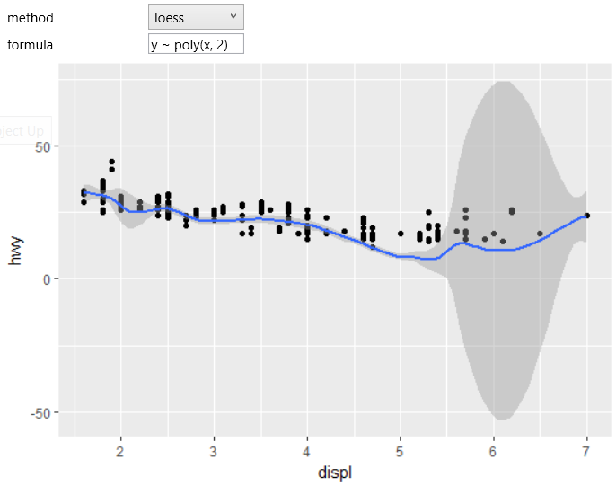
Another example shows using the method of local polynomial
regression smoothing (loess) with polynomial formula.
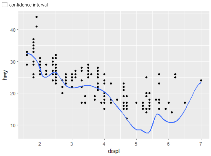
If you don't want to display the confidence interval, just set
the check-box (with the same name) to FALSE.
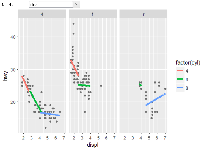
Finally, the last example shows how to use the geom_smooth
layer along with other objects. In the following graph we
used the geom_smooth layer on the dataset that was divided
according to the variable factor(cyl) into three groups
(color aes) and the visualization was faceted (facet_wrap
object) into separate graphs by the categorical variable
drv. In the result, we Plot the patterns between displ
and hwy variables that are broken down into groups by two
variables – cyl and drv.
For displaying the smoothing lines, you can use one more
object – stat_smooth statistical layer, which also allows
you to define additional auxiliary properties. Its description
can be found in the next chapter, which deals with defining
and setting statistical layers.