 geom_bind2d
geom_bin2d divides 2D plane into rectangles, counts the number of cases in
each rectangle, and then (by default) maps the number of cases to the
rectangle's fill. This is a useful alternative to geom_point in the
presence of overplotting.
Aesthetics
Other Properties
| bins |
numeric vector giving number of bins in both vertical and horizontal directions. Set to 30 by default |
| binwidth |
numeric vector giving bin width in both vertical and horizontal directions. Overrides bins if both set |
| drop |
if TRUE, removes all cells with 0 counts |
Computed Variables
| count |
number of points in bin |
| density |
density estimate |
| ncount |
count, scaled to maximum of 1 |
| ndensity |
density estimate, scaled to maximum of 1 |
Similar Geometries
geom_hex,
geom_density2D
Description and Details
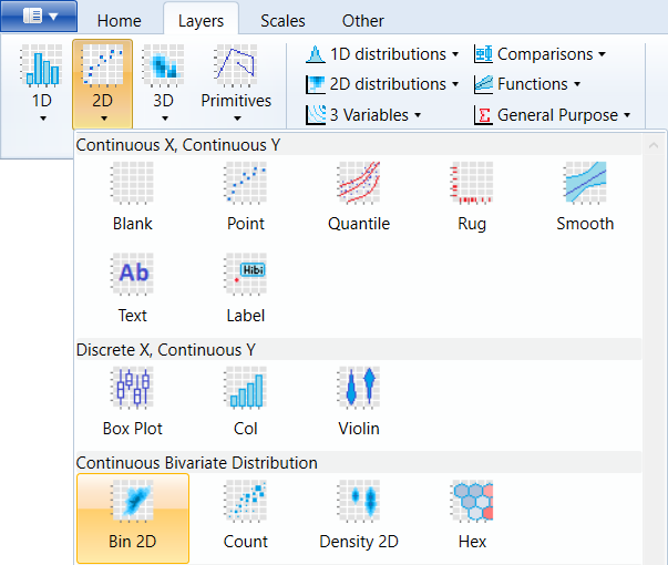
Using the described geometry, you can insert a simple geometric object
into your data visualization – a rectangles defined by a position
aesthetics properties (x and y) and count computed variable. You
can find this geometry in the ribbon toolbar tab Layers, under
the 2D button.
geom_bin2d is most commonly used to display continuous bivariate distribution.
For example, we use diamonds dataset that contains over 60,000 records.
An example of the relationship between the price of diamonds and carats is
shown in the following figure.
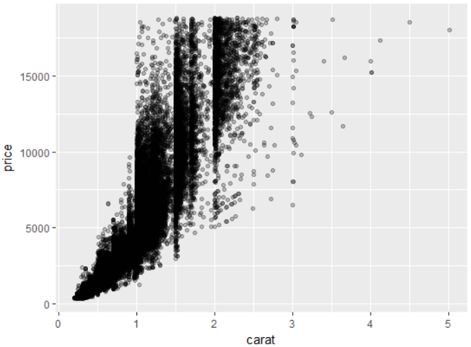
In this case, we see significant overplotting. The 2D distribution can be
viewed using geom_bin2d geometry. In this case, the area of the chart is
divided into squares and the number of points is calculated under each
square. This number is then mapped as a Computed Variable to aesthetic
property fill. The example is shown in the following figure. For definition,
simply select the dataset and map variables to the aesthetic positional
properties x and y.
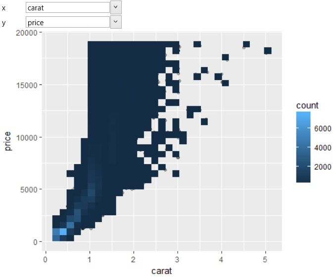
The program automatically generates 30 bins. This number is not always
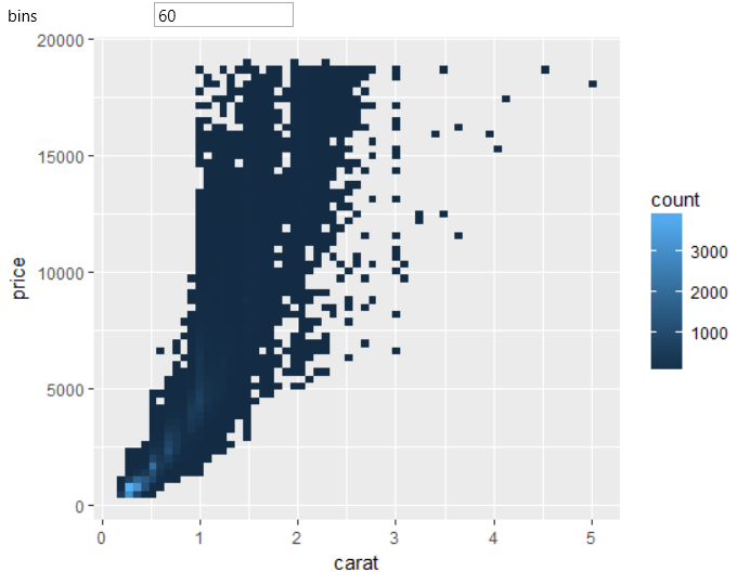
appropriate. That's why you can redefine this number using the bins property.
In the following figure, we changed the bins parameter to 60, which means
that the program creates a double number of rectangles.
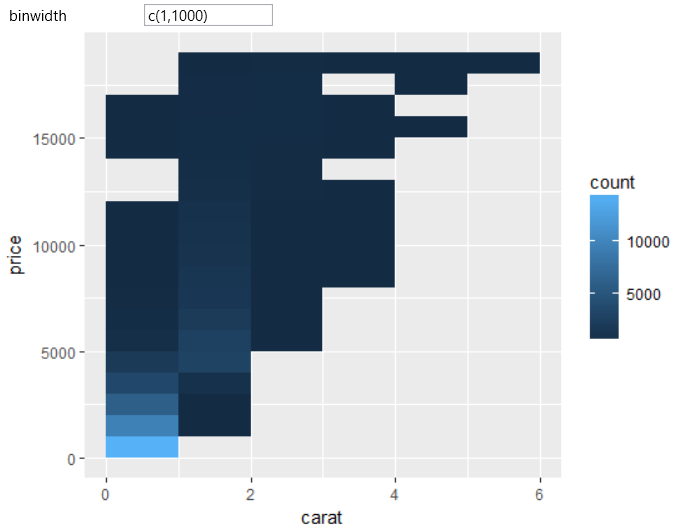
The second method for bins defining is the binwidth property. If you define
both properties (bin & binwidth), program uses bindwidth. If you use the
binwidth, you need to define the width and height of the rectangle. These
two values are defined in c() function. The example is shown in the
following figure. From this example it is clear that the width and
height of rectangles may vary.
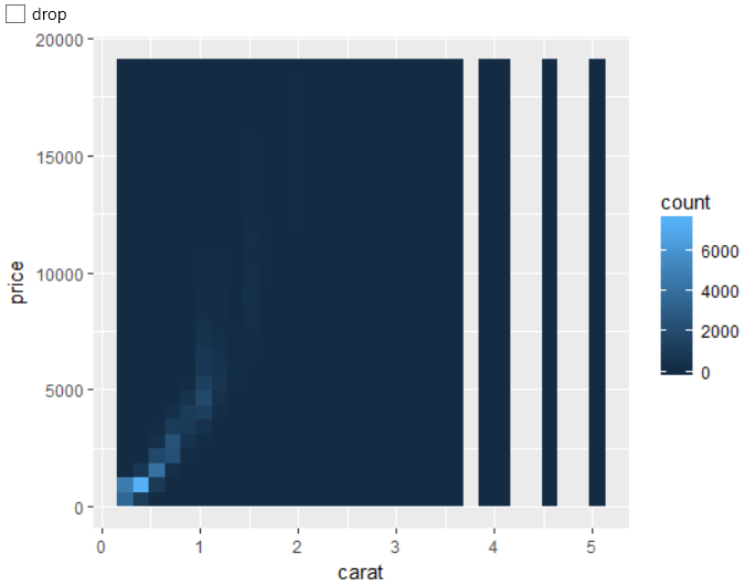
Under Properties section is one more property – drop. By default, it is
set to TRUE and this means that all rectangles without points are deleted.
If you set drop to FALSE, all cells are displayed in plot.
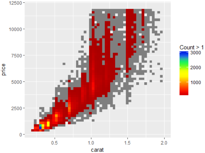
More options you can apply if you use described geometry along with object
from scale_fill group. For example, the following figure shows geom_bin2d
layer with scale_fill_gradient object. We use the color scale to display
geometry layer in rainbow palette and this scale was applied to cells
where count > 1. All rectangles with 1 point are shown in gray (na.value
property).
Similarly, you can use geom_hex layer. This geometry is defined in the
same way, but result values are rendered in hexagons.